- Published on
K-means 聚类算法:从理论到图像压缩
- Authors

- Name
- Allen Wang
在这篇博客中,我们将从零开始实现 K-means 算法,探索它如何将数据分组为簇,并将其应用于图像压缩,将一张彩色图片的颜色数量从数千种减少到仅 16 种。
目录
1 - 实现 K-means 算法
K-means 是一种无监督学习算法,用于将相似的数据点自动分组为簇。想象你有一堆散乱的珠子,想把它们按颜色或大小整理成几堆,这就是 K-means 的工作原理!具体来说,它的工作流程如下:
- 随机猜测初始的簇中心(称为 质心 或 centroids)。
- 不断重复两个步骤,直到质心稳定:
- 将每个数据点分配到离它最近的质心。
- 根据分配的点,更新每个质心的位置为这些点的平均位置。
K-means 伪代码
# 初始化质心
centroids = kMeans_init_centroids(X, K)

# 循环固定次数
for iter in range(iterations):
    # 步骤 1:将数据点分配到最近的质心
    idx = find_closest_centroids(X, centroids)
    # 步骤 2:根据分配更新质心位置
    centroids = compute_centroids(X, idx, K)
我们将分两部分实现这个算法:寻找最近的质心和更新质心位置。
1.1 寻找最近的簇中心
在 簇分配 阶段,K-means 算法为每个数据点找到离它最近的质心,并记录质心的索引。
练习 1:实现 find_closest_centroids
我们需要实现以下功能:
- 输入: 数据矩阵
X(形状为(m, n),其中m是数据点数量,n是特征数量)和质心矩阵centroids(形状为(K, n),其中K是簇数量)。 - 输出: 数组
idx(形状为(m,)),记录每个数据点最近的质心索引(0 到K-1)。
对于每个数据点 ,我们找到使其距离最小的质心 :
- 距离定义为欧氏距离的平方:
代码如下:
import numpy as np

def find_closest_centroids(X, centroids):
    """
    为每个数据点分配最近的质心。

    参数:
        X (ndarray): 形状 (m, n),数据点
        centroids (ndarray): 形状 (K, n),质心

    返回:
        idx (array_like): 形状 (m,),每个数据点的最近质心索引
    """
    K = centroids.shape[0]
    idx = np.zeros(X.shape[0], dtype=int)

    for i in range(X.shape[0]):
        distances = []
        for j in range(K):
            # 计算数据点 X[i] 到质心 j 的欧氏距离
            norm_ij = np.linalg.norm(X[i] - centroids[j])
            distances.append(norm_ij)
        # 选择距离最小的质心索引
        idx[i] = np.argmin(distances)

    return idx
代码详解:
np.linalg.norm(X[i] - centroids[j])计算点和质心之间的欧氏距离。np.argmin(distances)返回最小距离对应的质心索引。- 循环遍历每个数据点,确保每个点都被正确分配。
测试代码: 为了直观理解,假设我们有一个小型数据集:
# 样例数据(2D 点)
X = np.array([[1.8, 4.6], [5.6, 4.8], [6.3, 3.3], [2.9, 4.6], [3.2, 4.9]])
initial_centroids = np.array([[3, 3], [6, 2], [8, 5]])
idx = find_closest_centroids(X, initial_centroids)
print("前三个数据点的最近质心索引:", idx[:3])
预期输出:
前三个数据点的最近质心索引: [0 2 1]
这表示第一个点分配到质心 0,第二个点到质心 2,第三个点到质心 1。
1.2 计算簇中心均值
在 质心更新 阶段,我们根据分配结果重新计算每个质心的位置,取分配到该质心的所有点的平均值。
练习 2:实现 compute_centroids
任务:
- 输入: 数据
X、分配索引idx和簇数量K。 - 输出: 更新后的质心矩阵(形状为
(K, n))。
对于每个质心 ,更新公式为:
- 取所有分配到簇 (k) 的点的平均值:
实现代码如下:
def compute_centroids(X, idx, K):
    """
    根据分配结果更新质心位置。

    参数:
        X (ndarray): 形状 (m, n),数据点
        idx (ndarray): 形状 (m,),质心分配索引
        K (int): 簇数量

    返回:
        centroids (ndarray): 形状 (K, n),更新后的质心
    """
    m, n = X.shape
    centroids = np.zeros((K, n))

    for k in range(K):
        # 获取分配到簇 k 的所有点
        points = X[idx == k]
        # 计算这些点的均值
        centroids[k] = np.mean(points, axis=0)

    return centroids
代码详解:
X[idx == k]筛选出分配到簇k的数据点。np.mean(points, axis=0)沿特征维度计算平均值,得到新的质心位置。- 如果某个簇为空(无点分配),
np.mean会返回NaN,在实际应用中需要处理(这里假设数据合理)。
测试代码: 使用之前的样例数据和分配结果:
K = 3
centroids = compute_centroids(X, idx, K)
print("更新后的质心:", centroids)
预期输出(基于完整数据集):
更新后的质心: [[2.42830111 3.15792418]
                 [5.81350331 2.63365645]
                 [7.11938687 3.6166844 ]]
这表示每个质心已移动到其簇的中心。
2 - 在样例数据集上运行 K-means
现在,我们将两个函数组合起来,在一个简单的 2D 数据集上运行 K-means,并可视化聚类过程。
以下是运行 K-means 的完整函数:
import matplotlib.pyplot as plt

def run_kMeans(X, initial_centroids, max_iters=10, plot_progress=False):
    """
    在数据集 X 上运行 K-means 算法。

    参数:
        X (ndarray): 形状 (m, n),数据点
        initial_centroids (ndarray): 形状 (K, n),初始质心
        max_iters (int): 最大迭代次数
        plot_progress (bool): 是否可视化过程

    返回:
        centroids (ndarray): 最终质心
        idx (ndarray): 数据点分配
    """
    m, n = X.shape
    K = initial_centroids.shape[0]
    centroids = initial_centroids
    idx = np.zeros(m)

    for i in range(max_iters):
        print(f"K-means 迭代 {i}/{max_iters-1}")
        idx = find_closest_centroids(X, centroids)
        if plot_progress:
            plt.scatter(X[:, 0], X[:, 1], c=idx, cmap='viridis')
            plt.scatter(centroids[:, 0], centroids[:, 1], c='red', marker='x', s=200)
            plt.title(f"迭代 {i}")
            plt.pause(0.5)
        centroids = compute_centroids(X, idx, K)
    if plot_progress:
        plt.show()
    return centroids, idx
运行示例: 使用假设的样例数据:
# 样例数据(5 个 2D 点)
X = np.array([[1.8, 4.6], [5.6, 4.8], [6.3, 3.3], [2.9, 4.6], [3.2, 4.9]])
initial_centroids = np.array([[3, 3], [6, 2], [8, 5]])
centroids, idx = run_kMeans(X, initial_centroids, max_iters=10, plot_progress=True)
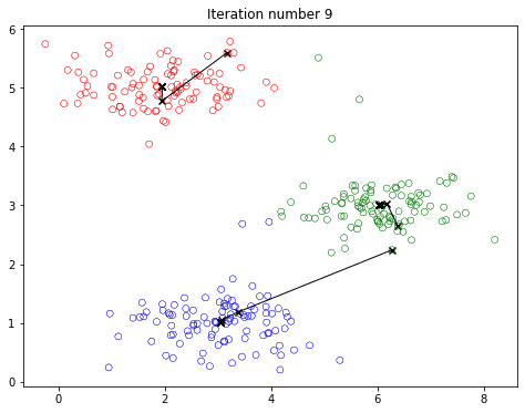
运行效果:
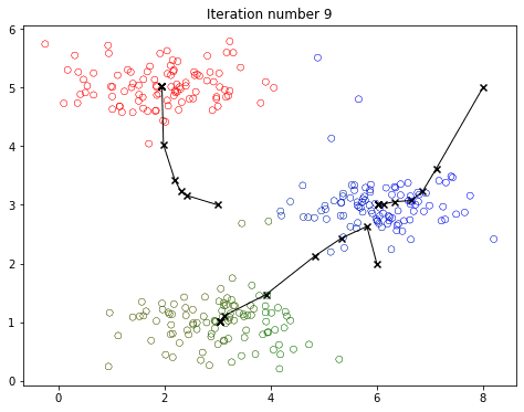
- 每次迭代,数据点会根据颜色(簇分配)分组,红色 X 标记表示质心。
- 质心逐步移动到簇的中心,最终稳定。
说明: 实际数据可能包含更多点(例如 300 个),效果更明显。这里用小型数据集便于理解。
3 - 随机初始化簇中心
初始质心的选择对 K-means 结果影响很大。一个好的策略是随机选择数据点作为初始质心。以下是实现:
def kMeans_init_centroids(X, K):
    """
    随机选择 K 个数据点作为初始质心。

    参数:
        X (ndarray): 数据点
        K (int): 簇数量

    返回:
        centroids (ndarray): 初始质心
    """
    randidx = np.random.permutation(X.shape[0])
    return X[randidx[:K]]
尝试一下: 多次运行以下代码,观察不同初始质心如何影响聚类结果:
K = 3
max_iters = 10
initial_centroids = kMeans_init_centroids(X, K)
centroids, idx = run_kMeans(X, initial_centroids, max_iters, plot_progress=True)
观察:
每次运行,质心的起始位置不同,可能导致不同的簇划分。这就是 K-means 的随机性!
4 - 使用 K-means 进行图像压缩
现在,我们将 K-means 应用到一个有趣的场景:图像压缩。通过将图像的颜色数量从数千种减少到 16 种,我们可以大幅减少存储空间,同时保留图像的主要特征。
4.1 图像数据集
我们将使用一张小鸟的图片(假设为 bird_small.png):
original_img = plt.imread('bird_small.png')
plt.imshow(original_img)
plt.title('原始图像')
plt.show()
print("图像形状:", original_img.shape)  # (128, 128, 3)
数据说明:
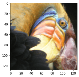
- 图像是一个 128×128 像素的矩阵,每个像素有 3 个通道(RGB),值在 0 到 1 之间(PNG 格式)。
- 每个像素是一个 3D 向量,例如
[0.5, 0.7, 0.2]表示红、绿、蓝强度。
4.2 对图像像素应用 K-means
为了应用 K-means,我们需要将图像展平为像素列表:
# 将图像展平为 (16384, 3) 的矩阵
X_img = np.reshape(original_img, (original_img.shape[0] * original_img.shape[1], 3))
然后运行 K-means,找到 16 个代表性颜色(簇):
K = 16
max_iters = 10
initial_centroids = kMeans_init_centroids(X_img, K)
centroids, idx = run_kMeans(X_img, initial_centroids, max_iters)
print("Shape of idx:", idx.shape)
print("Closest centroid for the first five elements:", idx[:5])
Shape of idx: (16384,) Closest centroid for the first five elements: [4 4 4 4 4]
# Plot the colors of the image and mark the centroids
plot_kMeans_RGB(X_img, centroids, idx, K)
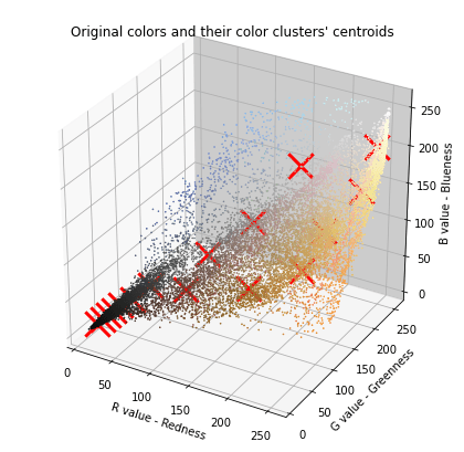
# Visualize the 16 colors selected
#你可以使用下面的函数可视化每个红色标记(即质心)处的颜色。只有在下一节生成新图像时,你才能看到这些颜色。每个颜色下方的数字是其索引,这些数字是你在 idx 数组中看到的数字。
show_centroid_colors(centroids)

运行效果:
centroids是 16 个 RGB 颜色(形状(16, 3))。idx记录每个像素所属的簇(0 到 15)。
4.3 压缩图像
现在,用每个像素的最近质心颜色替换原始颜色:
# 为每个像素分配最近的质心颜色
idx = find_closest_centroids(X_img, centroids)
X_recovered = centroids[idx, :]
# 恢复图像形状
X_recovered = np.reshape(X_recovered, original_img.shape)

# 显示原始和压缩图像
fig, ax = plt.subplots(1, 2, figsize=(8, 4))
ax[0].imshow(original_img)
ax[0].set_title('原始图像')
ax[0].axis('off')
ax[1].imshow(X_recovered)
ax[1].set_title('压缩图像(16 种颜色)')
ax[1].axis('off')
plt.show()
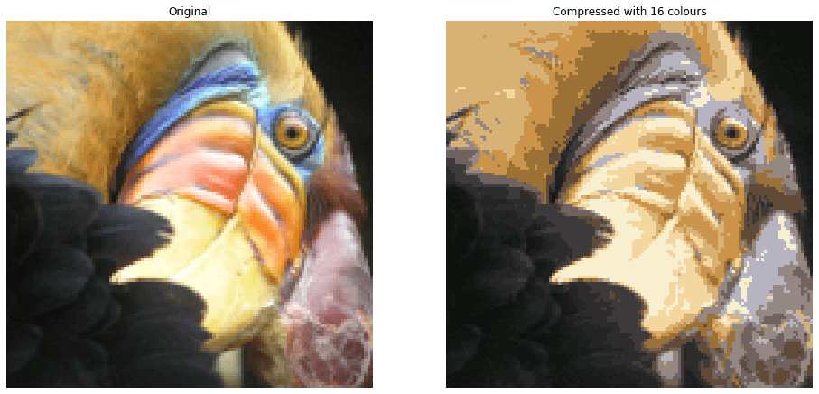
压缩原理:
- 原始图像: 128 × 128 × 24 位 = 393,216 位。
- 压缩图像: 16 种颜色 × 24 位 + 128 × 128 × 4 位 = 65,920 位,压缩约 6 倍!
- 每个像素只需存储一个 4 位索引(指向 16 种颜色之一),大大节省空间。
效果: 压缩后的图像保留了主要特征,但由于颜色减少,可能会出现轻 细微的压缩伪影(如颜色过渡不自然)。尝试调整 K 或 max_iters 来观察效果变化!
5 - 交互式可视化探索
5.1 怎么选 K 才更稳妥?
给新手一个实用流程:
- 先画 Elbow 曲线,找“拐点候选区”
- 在候选区比较 Silhouette 分数
- 最终结合业务可解释性选 K(例如推荐分群希望 4~8 类)
5.2 常见排错建议
- 如果结果每次差异很大:固定随机种子并增加初始化次数(
n_init) - 如果某些簇空了:检查初始化或降低 K
- 如果收敛慢:先做特征缩放、减少噪声维度
总结
恭喜你完成了这场 K-means 聚类的实践之旅!通过这篇博客,你学会了:
- 从零实现 K-means 算法,包括分配和更新质心。
- 在 2D 数据集上运行 K-means 并可视化聚类过程。
- 将 K-means 应用于图像压缩,减少颜色数量并保留图像特征。
希望这篇文章为你打开了机器学习聚类的大门!想进一步探索?试试用不同的 K 值或自己的图片,看看效果如何。下期我们将探讨无监督学习的另一个应用:异常检测,敬请期待!
完整代码已开源在GitHub仓库
本篇文章的部分内容和思想参考了 吴恩达 (Andrew Ng) 在 Coursera 机器学习课程 中的讲解,感谢他对机器学习领域的卓越贡献。