决策树实战：从零构建蘑菇分类器

在这篇博客中，我们将一起动手实现一个决策树，从头构建一个模型，用来判断蘑菇是可食用还是有毒。想象一下，你将用简单的规则，把杂乱的数据变成清晰的分类决策——这正是决策树的魅力所在！无论你是机器学习新手还是想复习基础，这篇文章都会带你一步步理解决策树的原理和实现。准备好了吗？让我们开始吧！

1 - 准备工具包

在动手之前，我们需要准备一些 Python 工具，它们是我们实现决策树的好帮手：

NumPy：处理数组和数学运算的利器，帮我们快速计算熵和信息增益。
Matplotlib：绘图工具，让我们把决策树和数据可视化，直观感受结果。
utils.py：一个辅助文件，包含一些现成的函数，比如加载数据和可视化树。我们不用改它，直接用就行。

运行以下代码，加载这些工具：

Python

import numpy as np
import matplotlib.pyplot as plt
from utils import *
%matplotlib inline

关于 utils.py：
你可以把 utils.py 想象成一个“工具箱”，里面有 load_data()（加载数据）和 generate_tree_viz()（画树）等函数。这些都是现成的，我们直接调用就好，不用自己从头写，省时又省力。

这些工具准备好后，我们就可以进入正题了！

2 - 问题背景

假设你开了一家野生蘑菇公司，专门种植和销售蘑菇。但有个问题：不是所有蘑菇都能吃，有的甚至有毒！为了安全起见，你希望根据蘑菇的外观特征（比如帽子的颜色、茎的形状、是否单独生长），判断它是否可食用。你已经收集了一些数据，接下来我们要用这些数据训练一个决策树模型，帮你快速分辨哪些蘑菇可以放心卖。

任务： 用决策树判断蘑菇是可食用（1）还是有毒（0）。

注意： 这只是个教学例子，真实生活中别靠这个数据集挑蘑菇吃哦！

3 - 数据集概览

让我们先加载数据集，看看我们要处理什么。以下是数据的一个样本：

数据包含 10 个蘑菇样本，每个样本有 3 个特征：
- 帽子颜色：棕色（Brown）或红色（Red）。
- 茎形状：变细（Tapering，像“/”）或变粗（Enlarging，像“/\”）。
- 是否单独生长：是（Yes）或否（No）。
标签：可食用（1）或有毒（0）。

3.1 独热编码数据集

为了让计算机更容易处理，我们把这些特征变成了“0”和“1”的形式（叫独热编码）。看下面转换后的数据：

X_train：特征矩阵，每行是一个样本，每列是一个特征（棕色帽子、变细茎、单独生长）。
y_train：标签数组，1 表示可食用，0 表示有毒。

加载数据：

Python

X_train = np.array([[1,1,1], [1,0,1], [1,0,0], [1,0,0], [1,1,1],
                    [0,1,1], [0,0,0], [1,0,1], [0,1,0], [1,0,0]])
y_train = np.array([1, 1, 0, 0, 1, 0, 0, 1, 1, 0])

探索数据

我们先打印数据，看看它长什么样：

Python

print("X_train 前五行:\n", X_train[:5])
print("X_train 类型:", type(X_train))

输出：

JavaScript

X_train 前五行:
 [[1 1 1]
  [1 0 1]
  [1 0 0]
  [1 0 0]
  [1 1 1]]
X_train 类型: <class 'numpy.ndarray'>

再看看标签：

Python

print("y_train 前五个元素:", y_train[:5])
print("y_train 类型:", type(y_train))

输出：

JavaScript

y_train 前五个元素: [1 1 0 0 1]
y_train 类型: <class 'numpy.ndarray'>

检查数据规模

用 shape 查看数据维度：

Python

print('X_train 形状:', X_train.shape)
print('y_train 形状:', y_train.shape)
print('样本数:', len(X_train))

输出：

JavaScript

X_train 形状: (10, 3)
y_train 形状: (10,)
样本数: 10

X_train 是 10 行 3 列的矩阵，10 个样本，每个样本 3 个特征。
y_train 是 10 个标签，和样本数对应。

4 - 决策树基础

决策树就像一个“问答游戏”：通过一系列问题，把数据分成不同的组，最终判断每个蘑菇是可食用还是有毒。构建决策树的过程是：

从根节点开始，包含所有样本。
计算每个特征的信息增益，选择增益最大的那个特征来分割。
根据选定的特征，把数据分成左右两个分支。
对每个分支重复这个过程，直到满足停止条件（比如达到最大深度）。

在这部分，我们将实现几个核心函数：

计算熵（衡量数据的混乱程度）。
分割数据集。
计算信息增益。
选择最佳分割特征。

我们设定最大深度为 2，也就是说树最多分两层。

4.1 计算熵

熵（entropy）是衡量数据“混乱度”的指标。如果一个节点里全是可食用的蘑菇（或全是有毒的），熵是 0；如果一半一半，熵最高。我们用它来判断分割前后的混乱度变化。

熵的公式是：

可食用比例是 p1，则熵 H(p1) = -p1 * log2(p1) - (1-p1) * log2(1-p1)。
特殊情况：如果 p1 = 0 或 1，熵设为 0（因为 0 * log(0) 定义为 0）。

动手练习 1：实现熵计算

完成下面的 compute_entropy 函数：

Python

def compute_entropy(y):
    """
    计算节点的熵。

    参数:
        y (ndarray): 节点样本的标签数组（1 表示可食用，0 表示有毒）

    返回:
        entropy (float): 熵值
    """
    entropy = 0.

    if len(y) != 0:  # 检查数据是否为空
        p1 = len(y[y == 1]) / len(y)  # 计算可食用比例
        if p1 != 0 and p1 != 1:  # 如果不是全 0 或全 1
            entropy = -p1 * np.log2(p1) - (1 - p1) * np.log2(1 - p1)
        else:
            entropy = 0.

    return entropy

代码详解：

len(y[y == 1])：计算标签为 1 的样本数。
p1：可食用比例，比如根节点有 5 个 1，5 个 0，则 p1 = 0.5。
熵公式：用 NumPy 的 np.log2 计算以 2 为底的对数。

测试一下： 在根节点（包含所有样本）计算熵：

Python

print("根节点熵:", compute_entropy(y_train))

输出：

JavaScript

根节点熵: 1.0

根节点有 5 个可食用，5 个有毒，p1 = 0.5，熵正好是 1，说明数据完全“混乱”，需要分割。

4.2 数据集分割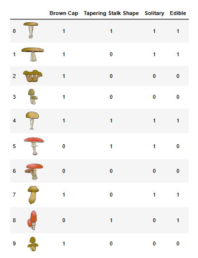

接下来，我们要实现一个函数，把数据按某个特征分成两组。比如，按“是否单独生长”分割，值为 1 的去左分支，值为 0 的去右分支。

动手练习 2：实现数据分割

完成 split_dataset 函数：

Python

def split_dataset(X, node_indices, feature):
    """
    根据特征分割数据集。

    参数:
        X (ndarray): 数据矩阵，形状 (样本数, 特征数)
        node_indices (list): 当前节点的样本索引
        feature (int): 要分割的特征索引

    返回:
        left_indices (list): 特征值为 1 的索引
        right_indices (list): 特征值为 0 的索引
    """
    left_indices = []
    right_indices = []

    for i in node_indices:
        if X[i][feature] == 1:
            left_indices.append(i)
        else:
            right_indices.append(i)

    return left_indices, right_indices

代码详解：

X[i][feature]：第 i 个样本的第 feature 个特征值。
如果值为 1，放进 left_indices；值为 0，放进 right_indices。

测试一下： 在根节点（所有样本）按特征 0（棕色帽子）分割：

Python

# Case 1
root_indices = [0, 1, 2, 3, 4, 5, 6, 7, 8, 9]
feature = 0
left_indices, right_indices = split_dataset(X_train, root_indices, feature)
print("左分支索引（棕色帽子）:", left_indices)
print("右分支索引（红色帽子）:", right_indices)
generate_split_viz(root_indices_subset, left_indices, right_indices, feature)
split_dataset_test(split_dataset)
# Case 2
root_indices_subset = [0, 2, 4, 6, 8]
feature = 0
left_indices, right_indices = split_dataset(X_train, root_indices, feature)
print("左分支索引（棕色帽子）:", left_indices)
print("右分支索引（红色帽子）:", right_indices)
generate_split_viz(root_indices_subset, left_indices, right_indices, feature)
split_dataset_test(split_dataset)

输出：

JavaScript

左分支索引（棕色帽子）: [0, 1, 2, 3, 4, 7, 9]
右分支索引（红色帽子）: [5, 6, 8]

JavaScript

左分支索引（棕色帽子）: [0, 2, 4]
右分支索引（红色帽子）: [6, 8]

棕色帽子（1）的样本去了左分支，红色帽子（0）的去了右分支。

4.3 计算信息增益

信息增益（Information Gain）衡量分割后数据混乱度的减少量。公式是：

信息增益 = 节点熵 - (左分支权重 _ 左分支熵 + 右分支权重 _ 右分支熵)。

动手练习 3：实现信息增益

完成 compute_information_gain 函数：

Python

def compute_information_gain(X, y, node_indices, feature):
    """
    计算按某特征分割的信息增益。

    参数:
        X (ndarray): 数据矩阵
        y (ndarray): 标签数组
        node_indices (list): 当前节点样本索引
        feature (int): 分割特征索引

    返回:
        information_gain (float): 信息增益
    """
    left_indices, right_indices = split_dataset(X, node_indices, feature)

    X_node, y_node = X[node_indices], y[node_indices]
    X_left, y_left = X[left_indices], y[left_indices]
    X_right, y_right = X[right_indices], y[right_indices]

    node_entropy = compute_entropy(y_node)
    left_entropy = compute_entropy(y_left)
    right_entropy = compute_entropy(y_right)

    w_left = len(X_left) / len(X_node)
    w_right = len(X_right) / len(X_node)

    weighted_entropy = w_left * left_entropy + w_right * right_entropy
    information_gain = node_entropy - weighted_entropy

    return information_gain

代码详解：

w_left 和 w_right：左右分支的样本比例。
weighted_entropy：加权后的分支熵。
信息增益：分割前熵减去加权后熵。

测试一下： 计算根节点按每个特征分割的信息增益：

Python

for feature in range(3):
    info_gain = compute_information_gain(X_train, y_train, root_indices, feature)
    print(f"特征 {feature} 的信息增益: {info_gain}")

输出：

JavaScript

特征 0 的信息增益: 0.034851554559677034
特征 1 的信息增益: 0.12451124978365313
特征 2 的信息增益: 0.2780719051126377

特征 2（单独生长）的增益最高，所以它是根节点的最佳分割特征。

4.4 选择最佳分割

现在，我们要找信息增益最大的特征，作为分割依据。

动手练习 4：找到最佳特征

完成 get_best_split 函数：

Python

def get_best_split(X, y, node_indices):
    """
    找到最佳分割特征。

    参数:
        X (ndarray): 数据矩阵
        y (ndarray): 标签数组
        node_indices (list): 当前节点样本索引

    返回:
        best_feature (int): 最佳特征索引
    """
    num_features = X.shape[1]
    best_feature = -1
    max_info_gain = 0

    for feature in range(num_features):
        info_gain = compute_information_gain(X, y, node_indices, feature)
        if info_gain > max_info_gain:
            max_info_gain = info_gain
            best_feature = feature

    return best_feature

测试一下：

Python

best_feature = get_best_split(X_train, y_train, root_indices)
print("最佳分割特征:", best_feature)

输出：

JavaScript

最佳分割特征: 2

特征 2（单独生长）被选中，和我们上面的分析一致。

5 - 构建决策树

有了以上函数，我们可以用递归的方式构建决策树。以下是现成的代码（无需修改），它会按最大深度 2 构建树并打印结果：

Python

tree = []
def build_tree_recursive(X, y, node_indices, branch_name, max_depth, current_depth):
    if current_depth == max_depth:
        print("  " * current_depth + f"{branch_name} 叶节点，索引: {node_indices}")
        return

    best_feature = get_best_split(X, y, node_indices)
    print("  " * current_depth + f"深度 {current_depth}, {branch_name}: 分割特征 {best_feature}")

    left_indices, right_indices = split_dataset(X, node_indices, best_feature)
    tree.append((left_indices, right_indices, best_feature))

    build_tree_recursive(X, y, left_indices, "左分支", max_depth, current_depth + 1)
    build_tree_recursive(X, y, right_indices, "右分支", max_depth, current_depth + 1)

build_tree_recursive(X_train, y_train, root_indices, "根节点", max_depth=2, current_depth=0)
generate_tree_viz(root_indices, y_train, tree)

输出：

JavaScript

深度 0, 根节点: 分割特征 2
  深度 1, 左分支: 分割特征 0
    左分支 叶节点，索引: [0, 1, 4, 7]
    右分支 叶节点，索引: [5]
  深度 1, 右分支: 分割特征 1
    左分支 叶节点，索引: [8]
    右分支 叶节点，索引: [2, 3, 6, 9]

可视化： 可以用 generate_tree_viz 画出树（需要 utils.py 支持），结果是一棵两层的决策树，根节点按“单独生长”分割，下一层分别按“棕色帽子”和“变细茎”分割。

6 - 交互式可视化探索

为了让“熵 → 信息增益 → 分裂策略”更直观，这里加入 3 个交互模块：

6.1 新手常见误区

误区1：信息增益越大越好，直接无限分裂
现实中会过拟合，需要限制深度或做剪枝。
误区2：训练集准确率高就代表模型好
要同时看验证集/测试集表现。
误区3：决策树不需要特征工程
脏数据、噪声特征仍会误导分裂。

总结

恭喜你完成了这场决策树实战！通过这篇博客，你学会了：

如何用熵衡量数据的混乱度。
如何按特征分割数据并计算信息增益。
如何选择最佳特征，递归构建决策树。

这棵树虽然简单，但已经能帮我们判断蘑菇的可食用性了！决策树是机器学习的基础，掌握它后，你可以进一步探索随机森林等高级模型。

完整代码已开源在GitHub仓库

本篇文章的部分内容和思想参考了吴恩达 (Andrew Ng) 在 Coursera 机器学习课程中的讲解，感谢他对机器学习领域的卓越贡献。

目录

1 - 准备工具包

2 - 问题背景

3 - 数据集概览

3.1 独热编码数据集

探索数据

检查数据规模

4 - 决策树基础

4.1 计算熵

动手练习 1：实现熵计算

4.2 数据集分割

动手练习 2：实现数据分割

4.3 计算信息增益

动手练习 3：实现信息增益

4.4 选择最佳分割

动手练习 4：找到最佳特征

5 - 构建决策树

6 - 交互式可视化探索

6.1 新手常见误区

总结