- Published on
机器学习模型评估与改进
- Authors

- Name
- Allen Wang
深入探讨如何评估和优化机器学习模型,特别是多项式回归和神经网络。通过理论讲解、代码实现和可视化分析,你将学会如何识别和解决过拟合与欠拟合问题,提升模型的泛化能力。
目录
1 - 准备工具包
在开始之前,我们需要导入一些 Python 工具包,它们将帮助我们完成数据处理、可视化和模型实现。运行下方代码以加载这些工具:
- NumPy:Python 中处理数组和矩阵运算的基础库。
- Matplotlib:一个强大的绘图库,用于生成数据可视化图表。
- Scikit-learn:一个用于数据挖掘和机器学习的库。
- TensorFlow:一个流行的机器学习平台。
import numpy as np
%matplotlib widget
import matplotlib.pyplot as plt
from sklearn.linear_model import LinearRegression, Ridge
from sklearn.preprocessing import StandardScaler, PolynomialFeatures
from sklearn.model_selection import train_test_split
from sklearn.metrics import mean_squared_error
import tensorflow as tf
from tensorflow.keras.models import Sequential
from tensorflow.keras.layers import Dense
from tensorflow.keras.activations import relu,linear
from tensorflow.keras.losses import SparseCategoricalCrossentropy
from tensorflow.keras.optimizers import Adam

import logging
logging.getLogger("tensorflow").setLevel(logging.ERROR)

tf.keras.backend.set_floatx('float64')
from assignment_utils import *

tf.autograph.set_verbosity(0)
这些工具是我们实现和评估机器学习模型的基石。
2 - 评估学习算法(多项式回归)
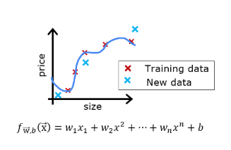
假设你已经创建了一个机器学习模型,并且发现它在训练数据上拟合得非常好。你完成了吗?还没那么快。创建模型的目的是能够预测新样本的值。
如何在部署模型之前测试其在新数据上的性能?答案有两部分:
- 将原始数据集分为“训练”和“测试”集。
- 使用训练数据拟合模型的参数。
- 使用测试数据评估模型在新数据上的性能。
- 开发一个误差函数来评估模型。
2.1 数据集分割
讲座中建议将 20-40% 的数据集保留为测试集。我们将使用 sklearn 的 train_test_split 函数来执行分割。运行以下代码后,请检查数据的形状。
# 生成一些数据
X, y, x_ideal, y_ideal = gen_data(18, 2, 0.7)
print("X.shape", X.shape, "y.shape", y.shape)

# 使用 sklearn 例程分割数据
X_train, X_test, y_train, y_test = train_test_split(X, y, test_size=0.33, random_state=1)
print("X_train.shape", X_train.shape, "y_train.shape", y_train.shape)
print("X_test.shape", X_test.shape, "y_test.shape", y_test.shape)
X.shape (18,) y.shape (18,) X_train.shape (12,) y_train.shape (12,) X_test.shape (6,) y_test.shape (6,)
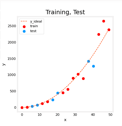
fig, ax = plt.subplots(1,1,figsize=(4,4))
ax.plot(x_ideal, y_ideal, "--", color = "orangered", label="y_ideal", lw=1)
ax.set_title("Training, Test",fontsize = 14)
ax.set_xlabel("x")
ax.set_ylabel("y")

ax.scatter(X_train, y_train, color = "red",           label="train")
ax.scatter(X_test, y_test,   color = dlc["dlblue"],   label="test")
ax.legend(loc='upper left')
plt.show()
2.2 模型评估的误差计算(线性回归)
在评估线性回归模型时,你需要计算预测值与目标值之间的平方误差差的平均值。
练习 1
请完成以下 eval_mse 函数,计算数据集上的均方误差。
def eval_mse(y, yhat):
    """
    计算数据集上的均方误差。
    参数:
        y (ndarray): 形状 (m,) 或 (m,1),每个样本的目标值
        yhat (ndarray): 形状 (m,) 或 (m,1),每个样本的预测值
    返回:
        err (scalar): 均方误差
    """
    m = len(y)
    err = 0.0
    for i in range(m):
        err_i = (yhat[i] - y[i]) ** 2
        err += err_i
    err = err / (2 * m)
    return err
2.3 比较训练和测试数据的性能
让我们构建一个高阶多项式模型来最小化训练误差。我们将使用 sklearn 的线性回归函数。以下是步骤:
- 创建并拟合模型(“拟合”是训练或运行梯度下降的另一种说法)。
- 计算训练数据上的误差。
- 计算测试数据上的误差。
# 在 sklearn 中创建一个模型,并在训练数据上训练
degree = 10
lmodel = lin_model(degree)
lmodel.fit(X_train, y_train)

# 预测训练数据,计算训练误差
yhat = lmodel.predict(X_train)
err_train = lmodel.mse(y_train, yhat)

# 预测测试数据,计算误差
yhat = lmodel.predict(X_test)
err_test = lmodel.mse(y_test, yhat)
print(f"training err {err_train:0.2f}, test err {err_test:0.2f}")
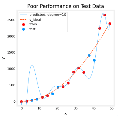
training err 58.01, test err 171215.01
训练集上的误差远小于测试集上的误差。以下图表显示了原因。模型非常好地拟合了训练数据,但为了做到这一点,它创建了一个复杂的函数。测试数据不是训练的一部分,模型在这些数据上的预测效果很差。这种模型可以描述为 1) 过拟合,2) 具有高方差,3) “泛化”能力差。
# 绘制预测曲线
x = np.linspace(0, int(X.max()), 100)
y_pred = lmodel.predict(x).reshape(-1, 1)

plt_train_test(X_train, y_train, X_test, y_test, x, y_pred, x_ideal, y_ideal, degree)
下表中显示的训练集、交叉验证集和测试集的分布是典型分布,但可能会因可用数据量而异。
| data 数据 | % of total 占总数的百分比 | Description 描述 |
|---|---|---|
| training 训练 | 60 | Data used to tune model parameters 𝑤w and 𝑏b in training or fitting 用于调整模型参数 𝑤w 以及 𝑏b 用于训练或拟合的数据 |
| cross-validation 交叉验证 | 20 | Data used to tune other model parameters like degree of polynomial, regularization or the architecture of a neural network. 用于调整其他模型参数的数据,例如多项式、正则化或神经网络的架构。 |
| test 测试 | 20 | Data used to test the model after tuning to gauge performance on new data 优化后用于测试模型以衡量新数据性能的数据 |
让我们在下面生成三个数据集。我们将再次使用 train_test_split from sklearn ,但将调用它两次以获得三个拆分:
# Generate  data
X,y, x_ideal,y_ideal = gen_data(40, 5, 0.7)
print("X.shape", X.shape, "y.shape", y.shape)

#split the data using sklearn routine
X_train, X_, y_train, y_ = train_test_split(X,y,test_size=0.40, random_state=1)
X_cv, X_test, y_cv, y_test = train_test_split(X_,y_,test_size=0.50, random_state=1)
print("X_train.shape", X_train.shape, "y_train.shape", y_train.shape)
print("X_cv.shape", X_cv.shape, "y_cv.shape", y_cv.shape)
print("X_test.shape", X_test.shape, "y_test.shape", y_test.shape)
X.shape (40,) y.shape (40,) X_train.shape (24,) y_train.shape (24,) X_cv.shape (8,) y_cv.shape (8,) X_test.shape (8,) y_test.shape (8,)
3 - 偏差与方差
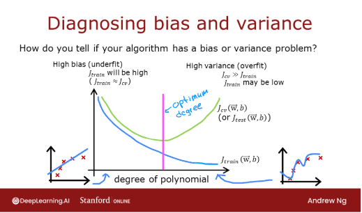
上面很明显,多项式模型的阶数过高。如何选择一个好的值?事实证明,如图所示,训练和交叉验证的性能可以提供指导。通过尝试一系列阶数值,可以评估训练和交叉验证的性能。随着阶数变得过大,交叉验证的性能将开始相对于训练性能下降。让我们在我们的示例中尝试这一点。
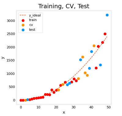
3.1 绘制训练、交叉验证和测试数据
你可以看到以下数据点,训练(红色)、交叉验证(橙色)和测试(蓝色)数据点是混在一起的。
fig, ax = plt.subplots(1, 1, figsize=(4, 4))
ax.plot(x_ideal, y_ideal, "--", color="orangered", label="y_ideal", lw=1)
ax.set_title("Training, CV, Test", fontsize=14)
ax.set_xlabel("x")
ax.set_ylabel("y")

ax.scatter(X_train, y_train, color="red", label="train")
ax.scatter(X_cv, y_cv, color="orange", label="cv")
ax.scatter(X_test, y_test, color="blue", label="test")
ax.legend(loc='upper left')
plt.show()
3.2 寻找最优多项式阶数
在之前的实验中,你发现可以通过使用多项式来创建能够拟合复杂曲线的模型。此外,你还展示了通过增加多项式的阶数,你可以“制造”过拟合。让我们在这里利用这些知识,测试我们区分过拟合和欠拟合的能力。
我们将反复训练模型,每次迭代增加多项式的阶数。在这里,我们将使用 scikit-learn 的线性回归模型以追求速度和简洁性。
max_degree = 9
err_train = np.zeros(max_degree)
err_cv = np.zeros(max_degree)
x = np.linspace(0, int(X.max()), 100)
y_pred = np.zeros((100, max_degree))

for degree in range(max_degree):
    lmodel = lin_model(degree + 1)
    lmodel.fit(X_train, y_train)
    yhat = lmodel.predict(X_train)
    err_train[degree] = lmodel.mse(y_train, yhat)
    yhat = lmodel.predict(X_cv)
    err_cv[degree] = lmodel.mse(y_cv, yhat)
    y_pred[:, degree] = lmodel.predict(x)

optimal_degree = np.argmin(err_cv) + 1
让我们绘制结果:
plt.close("all")
plt_optimal_degree(X_train, y_train, X_cv, y_cv, x, y_pred, x_ideal, y_ideal,
                   err_train, err_cv, optimal_degree, max_degree)
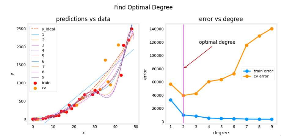
上述图表展示了将数据分为训练和未训练集可以帮助我们判断模型是欠拟合还是过拟合。在我们的示例中,我们通过增加多项式的阶数创建了从欠拟合到过拟合的各种模型。
- 左侧图表中,实线代表这些模型的预测。阶数为 1 的多项式模型产生一条直线,几乎不穿过数据点,而最大阶数的模型则非常贴合每个数据点。
- 右侧图表中:
- 训练数据的误差(蓝色)随着模型复杂度的增加而减小,这在意料之中。
- 交叉验证数据的误差最初随着模型开始适应数据而减小,但随着模型开始在训练数据上过拟合(未能“泛化”)而增加。
值得注意的是,这些示例中的曲线并不像讲座中那样平滑。这是可以预期的。重要的是总体趋势:随着模型复杂度的增加,训练误差减小,而交叉验证误差先减后增。
3.3 调整正则化
在之前的实验中,你利用正则化来减少过拟合。与阶数类似,你可以使用相同的方法来调整正则化参数 λ。
让我们通过从高阶多项式开始,并改变正则化参数来演示这一点。
lambda_range = np.array([0.0, 1e-6, 1e-5, 1e-4, 1e-3, 1e-2, 1e-1, 1, 10, 100])
num_steps = len(lambda_range)
degree = 10
err_train = np.zeros(num_steps)
err_cv = np.zeros(num_steps)
x = np.linspace(0, int(X.max()), 100)
y_pred = np.zeros((100, num_steps))

for i in range(num_steps):
    lambda_ = lambda_range[i]
    lmodel = lin_model(degree, regularization=True, lambda_=lambda_)
    lmodel.fit(X_train, y_train)
    yhat = lmodel.predict(X_train)
    err_train[i] = lmodel.mse(y_train, yhat)
    yhat = lmodel.predict(X_cv)
    err_cv[i] = lmodel.mse(y_cv, yhat)
    y_pred[:, i] = lmodel.predict(x)

optimal_reg_idx = np.argmin(err_cv)
plt.close("all")
plt_tune_regularization(X_train, y_train, X_cv, y_cv, x, y_pred, err_train, err_cv, optimal_reg_idx, lambda_range)
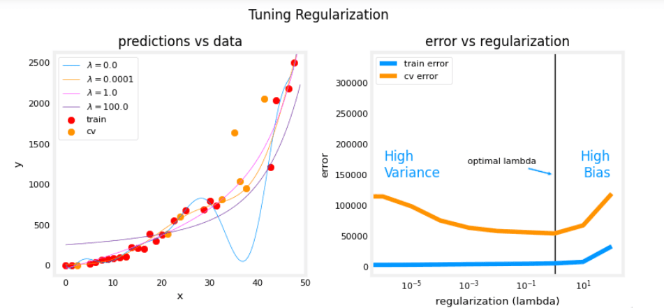
上述图表显示,随着正则化的增加,模型从高方差(过拟合)模型转变为高偏差(欠拟合)模型。右侧图表中的垂直线显示了 λ 的最优值。在这个示例中,多项式阶数设置为 10。
3.4 获取更多数据:增加训练集规模
当模型过拟合(高方差)时,收集更多数据可以提高性能。让我们在这里尝试。
X_train, y_train, X_cv, y_cv, x, y_pred, err_train, err_cv, m_range, degree = tune_m()
plt_tune_m(X_train, y_train, X_cv, y_cv, x, y_pred, err_train, err_cv, m_range, degree)
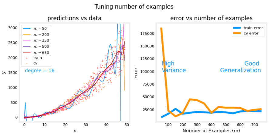
上述图表显示,当模型具有高方差并过拟合时,增加样本数量可以提高性能。请注意左侧图表中的曲线。具有最高 m 值的最终曲线是一条平滑的曲线,位于数据的中心。在右侧,随着样本数量的增加,训练集和交叉验证集的性能收敛到相似的值。请注意,曲线并不像讲座中那样平滑。这是可以预期的。趋势仍然清晰:更多数据可以改善泛化。
注意: 当模型具有高偏差(欠拟合)时,增加样本数量并不能改善性能。
4 - 评估学习算法(神经网络)
在上一节中,你调整了多项式回归模型的参数。现在,我们将转向神经网络模型。让我们从创建一个分类数据集开始。
4.1 数据集
运行以下代码,生成数据集并将其分为训练、交叉验证(CV)和测试集。在这个示例中,我们增加了交叉验证数据点的百分比以强调其重要性。
# 生成和分割数据集
X, y, centers, classes, std = gen_blobs()

# 分割数据。较大的 CV 群体以供演示
X_train, X_, y_train, y_ = train_test_split(X, y, test_size=0.50, random_state=1)
X_cv, X_test, y_cv, y_test = train_test_split(X_, y_, test_size=0.20, random_state=1)
print("X_train.shape:", X_train.shape, "X_cv.shape:", X_cv.shape, "X_test.shape:", X_test.shape)
X_train.shape: (400, 2) X_cv.shape: (320, 2) X_test.shape: (80, 2)
plt_train_eq_dist(X_train, y_train, classes, X_cv, y_cv, centers, std)
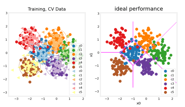
在左侧图表中,你可以看到数据点按颜色分为六个簇。训练点(圆点)和交叉验证点(三角形)都显示出来。有趣的是那些落在模糊位置的点,任何簇都可能将它们视为成员。你期望神经网络模型会如何处理?什么是过拟合和欠拟合的例子?
在右侧是一个“理想”模型的示例,或者是一个知道数据来源的人可能会创建的模型。线条代表“等距离”边界,其中到中心点的距离相等。值得注意的是,这个模型会“误分类”大约 8% 的总数据集。
4.2 通过计算分类误差评估分类模型
分类模型的评估函数很简单:不正确预测的比例。
练习 2
请完成以下 eval_cat_err 函数,计算分类误差。注意,在这个实验中,目标值是类别的索引,而不是one-hot 编码。
def eval_cat_err(y, yhat):
    """
    计算分类误差。
    参数:
        y (ndarray): 形状 (m,) 或 (m,1),每个样本的目标值
        yhat (ndarray): 形状 (m,) 或 (m,1),每个样本的预测值
    返回:
        cerr (scalar): 分类误差
    """
    m = len(y)
    incorrect = 0
    for i in range(m):
        if yhat[i] != y[i]:
            incorrect += 1
    cerr = incorrect / m
    return cerr
y_hat = np.array([1, 2, 0])
y_tmp = np.array([1, 2, 3])
print(f"categorization error {np.squeeze(eval_cat_err(y_hat, y_tmp)):0.3f}, expected:0.333" )
y_hat = np.array([[1], [2], [0], [3]])
y_tmp = np.array([[1], [2], [1], [3]])
print(f"categorization error {np.squeeze(eval_cat_err(y_hat, y_tmp)):0.3f}, expected:0.250" )

test_eval_cat_err(eval_cat_err)
categorization error 0.333, expected:0.333 categorization error 0.250, expected:0.250
5 - 模型复杂度
接下来,你将构建两个模型:一个复杂模型和一个简单模型。你将评估这些模型,以确定它们是过拟合还是欠拟合。
练习 3
请完成以下代码,构建一个三层模型:
- 具有 120 个单元的 Dense 层,relu 激活
- 具有 40 个单元的 Dense 层,relu 激活
- 具有 6 个单元的 Dense 层,线性激活(不是 softmax)
使用以下配置编译模型:
- 损失函数为
SparseCategoricalCrossentropy,记得使用from_logits=True - Adam 优化器,学习率为 0.01
tf.random.set_seed(1234)
model = Sequential(
    [
        Dense(120, activation='relu', name="L1"),
        Dense(40, activation='relu', name="L2"),
        Dense(classes, activation='linear', name="L3")
    ], name="Complex"
)
model.compile(
    loss=tf.keras.losses.SparseCategoricalCrossentropy(from_logits=True),
    optimizer=tf.keras.optimizers.Adam(0.01),
)
model.fit(X_train, y_train, epochs=1000)
model.summary()
model_test(model, classes, X_train.shape[1])
Model: "Complex"
_________________________________________________________________
 Layer (type)                Output Shape              Param #
=================================================================
 L1 (Dense)                  (None, 120)               360

 L2 (Dense)                  (None, 40)                4840

 L3 (Dense)                  (None, 6)                 246

=================================================================
Total params: 5,446
Trainable params: 5,446
Non-trainable params: 0
_________________________________________________________________
这个模型非常努力地捕捉每个类别的离群点。结果,它错误分类了一些交叉验证数据。让我们计算分类误差。
training_cerr_complex = eval_cat_err(y_train, model_predict(X_train))
cv_cerr_complex = eval_cat_err(y_cv, model_predict(X_cv))
print(f"分类误差,训练,复杂模型: {training_cerr_complex:0.3f}")
print(f"分类误差,CV,复杂模型: {cv_cerr_complex:0.3f}")
categorization error, training, complex model: 0.003 categorization error, cv, complex model: 0.122
5.1 简单模型
现在,尝试一个简单模型。
练习 4
请完成以下代码,构建一个两层模型:
- 具有 6 个单元的 Dense 层,relu 激活
- 具有 6 个单元的 Dense 层,线性激活
使用以下配置编译模型:
- 损失函数为
SparseCategoricalCrossentropy,使用from_logits=True - Adam 优化器,学习率为 0.01
tf.random.set_seed(1234)
model_s = Sequential(
    [
        Dense(6, activation='relu', name="L1"),
        Dense(classes, activation='linear', name="L2")
    ], name="Simple"
)
model_s.compile(
    loss=tf.keras.losses.SparseCategoricalCrossentropy(from_logits=True),
    optimizer=tf.keras.optimizers.Adam(0.01),
)
model_s.fit(X_train, y_train, epochs=1000)
model_s.summary()
model_s_test(model_s, classes, X_train.shape[1])
#make a model for plotting routines to call
model_predict_s = lambda Xl: np.argmax(tf.nn.softmax(model_s.predict(Xl)).numpy(),axis=1)
plt_nn(model_predict_s,X_train,y_train, classes, X_cv, y_cv, suptitle="Simple Model")
Model: "Simple"
_________________________________________________________________
 Layer (type)                Output Shape              Param #
=================================================================
 L1 (Dense)                  (None, 6)                 18

 L2 (Dense)                  (None, 6)                 42

=================================================================
Total params: 60
Trainable params: 60
Non-trainable params: 0
_________________________________________________________________
这个简单模型表现得相当不错。让我们计算分类误差。
training_cerr_simple = eval_cat_err(y_train, model_predict_s(X_train))
cv_cerr_simple = eval_cat_err(y_cv, model_predict_s(X_cv))
print(f"分类误差,训练,简单模型: {training_cerr_simple:0.3f}, 复杂模型: {training_cerr_complex:0.3f}")
print(f"分类误差,CV,简单模型: {cv_cerr_simple:0.3f}, 复杂模型: {cv_cerr_complex:0.3f}")
categorization error, training, simple model, 0.062, complex model: 0.003 categorization error, cv, simple model, 0.087, complex model: 0.122
我们的简单模型在训练集上的分类误差略高,但在交叉验证集上的表现优于更复杂的模型。
6 - 正则化
与多项式回归一样,可以应用正则化来调节更复杂模型的影响。让我们尝试在下面这样做。
练习 5
请重建你的复杂模型,但这次包含正则化。构建一个三层模型:
- 具有 120 个单元的 Dense 层,relu 激活,
kernel_regularizer=tf.keras.regularizers.l2(0.1) - 具有 40 个单元的 Dense 层,relu 激活,
kernel_regularizer=tf.keras.regularizers.l2(0.1) - 具有 6 个单元的 Dense 层,线性激活
使用以下配置编译模型:
- 损失函数为
SparseCategoricalCrossentropy,使用from_logits=True - Adam 优化器,学习率为 0.01
tf.random.set_seed(1234)
model_r = Sequential(
    [
        Dense(120, activation='relu', kernel_regularizer=tf.keras.regularizers.l2(0.1), name="L1"),
        Dense(40, activation='relu', kernel_regularizer=tf.keras.regularizers.l2(0.1), name="L2"),
        Dense(classes, activation='linear', name="L3")
    ], name="ComplexRegularized"
)
model_r.compile(
    loss=tf.keras.losses.SparseCategoricalCrossentropy(from_logits=True),
    optimizer=tf.keras.optimizers.Adam(0.01),
)
model_r.fit(X_train, y_train, epochs=1000)
model_r.summary()
model_r_test(model_r, classes, X_train.shape[1])
Model: "sequential"
_________________________________________________________________
 Layer (type)                Output Shape              Param #
=================================================================
 L1 (Dense)                  (None, 120)               360

 L2 (Dense)                  (None, 40)                4840

 L3 (Dense)                  (None, 6)                 246

=================================================================
Total params: 5,446
Trainable params: 5,446
Non-trainable params: 0
_________________________________________________________________
#make a model for plotting routines to call
model_predict_r = lambda Xl: np.argmax(tf.nn.softmax(model_r.predict(Xl)).numpy(),axis=1)
plt_nn(model_predict_r, X_train,y_train, classes, X_cv, y_cv, suptitle="Regularized")
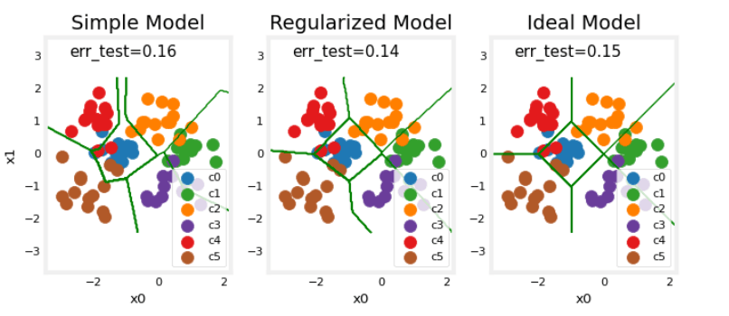
结果看起来与“理想”模型非常相似。让我们检查分类误差。
training_cerr_reg = eval_cat_err(y_train, model_predict_r(X_train))
cv_cerr_reg = eval_cat_err(y_cv, model_predict_r(X_cv))
print(f"分类误差,训练,正则化模型: {training_cerr_reg:0.3f}, 简单模型: {training_cerr_simple:0.3f}, 复杂模型: {training_cerr_complex:0.3f}")
print(f"分类误差,CV,正则化模型: {cv_cerr_reg:0.3f}, 简单模型: {cv_cerr_simple:0.3f}, 复杂模型: {cv_cerr_complex:0.3f}")
categorization error, training, regularized: 0.072, simple model, 0.062, complex model: 0.003 categorization error, cv, regularized: 0.066, simple model, 0.087, complex model: 0.122
简单模型在训练集上的分类误差略高,但在交叉验证集上的表现优于正则化模型。
7 - 迭代寻找最优正则化值
你可以尝试许多正则化值。以下代码需要几分钟才能运行。如果你有时间,可以运行并检查结果。如果没有,你已经完成了作业的评分部分!
tf.random.set_seed(1234)
lambdas = [0.0, 0.001, 0.01, 0.05, 0.1, 0.2, 0.3]
models = [None] * len(lambdas)

for i in range(len(lambdas)):
    lambda_ = lambdas[i]
    models[i] = Sequential(
        [
            Dense(120, activation='relu', kernel_regularizer=tf.keras.regularizers.l2(lambda_)),
            Dense(40, activation='relu', kernel_regularizer=tf.keras.regularizers.l2(lambda_)),
            Dense(classes, activation='linear')
        ]
    )
    models[i].compile(
        loss=tf.keras.losses.SparseCategoricalCrossentropy(from_logits=True),
        optimizer=tf.keras.optimizers.Adam(0.01),
    )
    models[i].fit(X_train, y_train, epochs=1000)
    print(f"完成 lambda = {lambda_}")
plot_iterate(lambdas, models, X_train, y_train, X_cv, y_cv)
随着正则化的增加,模型在训练和交叉验证数据集上的性能趋于收敛。对于这个数据集和模型,λ > 0.01 似乎是一个合理的选择。
7.1 测试
让我们在测试集上尝试我们优化的模型,并将其与“理想”性能进行比较。
plt_compare(X_test, y_test, classes, model_predict_s, model_predict_r, centers)
我们的测试集很小,并且似乎有许多离群点,因此分类误差很高。然而,我们优化模型的性能与理想性能相当。
8 - 交互式可视化探索
为了更直观地理解偏差-方差权衡和正则化效果,我们准备了三个交互式可视化工具:
8.1 偏差-方差权衡可视化
这个可视化展示了模型复杂度如何影响偏差和方差:
- 调整多项式阶数观察欠拟合到过拟合的转变
- 理解训练误差和验证误差的变化规律
- 找到最优模型复杂度的"甜蜜点"
8.2 正则化效果动画
实时观察正则化参数λ的影响:
- λ=0时的过拟合现象
- λ增大时模型逐渐平滑
- λ过大导致的欠拟合
- 学习曲线的动态变化
8.3 学习曲线3D可视化
通过3D视角理解训练集大小的影响:
- 小数据集时的高方差问题
- 数据增加如何改善泛化能力
- 识别是否需要更多数据
9 - 深入理解模型诊断
9.1 偏差-方差分解的数学原理
期望泛化误差分解:
其中:
- 偏差(Bias):模型预测的期望值与真实值的差距
- 方差(Variance):模型预测的波动程度
- 不可约误差:数据本身的噪声
实际应用:
def bias_variance_decomposition(model, X_train, y_train, X_test, y_test, n_iterations=100):
    """
    通过Bootstrap采样估计偏差和方差
    """
    predictions = []

    for i in range(n_iterations):
        # Bootstrap采样
        indices = np.random.choice(len(X_train), len(X_train), replace=True)
        X_boot = X_train[indices]
        y_boot = y_train[indices]

        # 训练模型
        model_copy = clone(model)
        model_copy.fit(X_boot, y_boot)
        predictions.append(model_copy.predict(X_test))

    predictions = np.array(predictions)

    # 计算偏差和方差
    mean_prediction = predictions.mean(axis=0)
    bias_squared = np.mean((mean_prediction - y_test) ** 2)
    variance = np.mean(predictions.var(axis=0))

    return bias_squared, variance

# 使用示例
from sklearn.base import clone
bias_sq, var = bias_variance_decomposition(model, X_train, y_train, X_cv, y_cv)
print(f"偏差²: {bias_sq:.4f}, 方差: {var:.4f}")
9.2 正则化的几何解释
L2正则化(Ridge):
# 目标函数
J(w) = MSE(w) + λ||w||²

# 等价于约束优化
minimize MSE(w)
subject to ||w||² ≤ t
几何意义:在权重空间中,L2正则化将解约束在一个球体内,鼓励权重均匀分布。
L1正则化(Lasso):
# 目标函数
J(w) = MSE(w) + λ||w||₁

# 等价于约束优化
minimize MSE(w)
subject to ||w||₁ ≤ t
几何意义:L1正则化将解约束在菱形内,容易产生稀疏解(部分权重为0),实现特征选择。
对比实验:
from sklearn.linear_model import Ridge, Lasso

# Ridge回归
ridge = Ridge(alpha=0.1)
ridge.fit(X_train, y_train)
print("Ridge权重:", ridge.coef_)

# Lasso回归
lasso = Lasso(alpha=0.1)
lasso.fit(X_train, y_train)
print("Lasso权重:", lasso.coef_)
print("非零权重数量:", np.sum(lasso.coef_ != 0))
9.3 交叉验证的高级技巧
K折交叉验证:
from sklearn.model_selection import KFold, cross_val_score

# 5折交叉验证
kfold = KFold(n_splits=5, shuffle=True, random_state=42)
scores = cross_val_score(model, X, y, cv=kfold, scoring='neg_mean_squared_error')

print(f"CV MSE: {-scores.mean():.4f} (+/- {scores.std():.4f})")
分层K折(用于分类):
from sklearn.model_selection import StratifiedKFold

# 保持类别比例的5折交叉验证
skfold = StratifiedKFold(n_splits=5, shuffle=True, random_state=42)
scores = cross_val_score(model, X, y, cv=skfold, scoring='accuracy')
时间序列交叉验证:
from sklearn.model_selection import TimeSeriesSplit

# 时间序列专用交叉验证(避免数据泄露)
tscv = TimeSeriesSplit(n_splits=5)
for train_idx, test_idx in tscv.split(X):
    X_train_fold, X_test_fold = X[train_idx], X[test_idx]
    y_train_fold, y_test_fold = y[train_idx], y[test_idx]
    # 训练和评估
10 - 常见问题与解决方案
问题1:如何判断是否需要更多数据?
学习曲线诊断:
from sklearn.model_selection import learning_curve

train_sizes, train_scores, val_scores = learning_curve(
    model, X, y, cv=5,
    train_sizes=np.linspace(0.1, 1.0, 10),
    scoring='neg_mean_squared_error'
)

plt.plot(train_sizes, -train_scores.mean(axis=1), label='训练误差')
plt.plot(train_sizes, -val_scores.mean(axis=1), label='验证误差')
plt.xlabel('训练集大小')
plt.ylabel('MSE')
plt.legend()
plt.show()
判断标准:
- ✅ 需要更多数据:训练误差和验证误差都很高,且随数据增加持续下降
- ❌ 不需要更多数据:验证误差已趋于平稳,增加数据无明显改善
问题2:正则化参数λ如何选择?
网格搜索:
from sklearn.model_selection import GridSearchCV

param_grid = {'alpha': np.logspace(-4, 4, 20)}
grid_search = GridSearchCV(Ridge(), param_grid, cv=5,
                           scoring='neg_mean_squared_error')
grid_search.fit(X_train, y_train)

print(f"最优λ: {grid_search.best_params_['alpha']:.4f}")
print(f"最优CV MSE: {-grid_search.best_score_:.4f}")
贝叶斯优化(更高效):
from skopt import BayesSearchCV

bayes_search = BayesSearchCV(
    Ridge(),
    {'alpha': (1e-4, 1e4, 'log-uniform')},
    n_iter=32,
    cv=5,
    scoring='neg_mean_squared_error'
)
bayes_search.fit(X_train, y_train)
问题3:神经网络过拟合严重怎么办?
综合解决方案:
from tensorflow.keras.layers import Dropout, BatchNormalization
from tensorflow.keras.regularizers import l2
from tensorflow.keras.callbacks import EarlyStopping, ReduceLROnPlateau

model = Sequential([
    Dense(128, activation='relu', kernel_regularizer=l2(0.01)),
    BatchNormalization(),  # 批归一化稳定训练
    Dropout(0.3),          # 30%神经元随机失活

    Dense(64, activation='relu', kernel_regularizer=l2(0.01)),
    BatchNormalization(),
    Dropout(0.2),

    Dense(10, activation='softmax')
])

# 早停法
early_stop = EarlyStopping(
    monitor='val_loss',
    patience=10,
    restore_best_weights=True
)

# 学习率衰减
lr_schedule = ReduceLROnPlateau(
    monitor='val_loss',
    factor=0.5,
    patience=5,
    min_lr=1e-6
)

model.compile(optimizer=Adam(learning_rate=0.001),
              loss='sparse_categorical_crossentropy',
              metrics=['accuracy'])

history = model.fit(X_train, y_train,
                    validation_data=(X_cv, y_cv),
                    epochs=100,
                    callbacks=[early_stop, lr_schedule])
问题4:多项式特征导致维度爆炸
特征选择:
from sklearn.feature_selection import SelectKBest, f_regression

# 生成多项式特征
poly = PolynomialFeatures(degree=5)
X_poly = poly.fit_transform(X)

# 选择最重要的K个特征
selector = SelectKBest(f_regression, k=20)
X_selected = selector.fit_transform(X_poly, y)

print(f"原始特征数: {X_poly.shape[1]}")
print(f"选择后特征数: {X_selected.shape[1]}")
主成分分析(PCA)降维:
from sklearn.decomposition import PCA

pca = PCA(n_components=0.95)  # 保留95%方差
X_pca = pca.fit_transform(X_poly)

print(f"降维后特征数: {X_pca.shape[1]}")
print(f"解释方差比: {pca.explained_variance_ratio_.sum():.2%}")
11 - 实战技巧总结
模型评估检查清单
# ✅ 数据分割检查
assert len(X_train) + len(X_cv) + len(X_test) == len(X), "数据分割错误"
assert 0.6 <= len(X_train)/len(X) <= 0.8, "训练集比例异常"

# ✅ 数据泄露检查
train_indices = set(range(len(X_train)))
cv_indices = set(range(len(X_train), len(X_train)+len(X_cv)))
assert train_indices.isdisjoint(cv_indices), "训练集和验证集有重叠!"

# ✅ 特征缩放检查
scaler = StandardScaler()
X_train_scaled = scaler.fit_transform(X_train)
X_cv_scaled = scaler.transform(X_cv)  # 注意:只用transform,不用fit
assert np.abs(X_train_scaled.mean()) < 0.1, "特征未正确标准化"

# ✅ 过拟合检查
train_error = mean_squared_error(y_train, model.predict(X_train))
cv_error = mean_squared_error(y_cv, model.predict(X_cv))
if cv_error > 2 * train_error:
    print("⚠️ 警告:模型可能过拟合!")
性能优化建议
向量化计算(避免Python循环):
Python# ❌ 慢速循环 errors = [] for i in range(len(X)): pred = model.predict(X[i:i+1]) errors.append((y[i] - pred) ** 2) # ✅ 向量化 predictions = model.predict(X) errors = (y - predictions) ** 2批量预测:
Python# 神经网络批量预测更快 predictions = model.predict(X_test, batch_size=128)缓存中间结果:
Pythonfrom functools import lru_cache @lru_cache(maxsize=128) def compute_polynomial_features(degree): poly = PolynomialFeatures(degree) return poly.fit_transform(X_train)
扩展学习方向
- 集成学习:结合多个模型(Bagging、Boosting、Stacking)
- 自动机器学习(AutoML):使用Auto-sklearn或TPOT自动调参
- 深度学习正则化:Dropout、Batch Normalization、Layer Normalization
- 迁移学习:利用预训练模型加速训练
总结
恭喜你完成了这篇关于机器学习模型评估和改进的实践博客!通过这次学习,你已经掌握了:
- 如何将数据分为训练和测试集,以区分欠拟合和过拟合。
- 如何创建训练、交叉验证和测试集,以训练模型参数、调整模型复杂度、正则化等,并评估模型在新数据上的性能。
- 如何通过比较训练和交叉验证的性能,洞察模型的过拟合(高方差)或欠拟合(高偏差)倾向。
希望这篇文章为你提供了宝贵的工具和见解,帮助你在未来的机器学习项目中取得成功!如果你想进一步探索,可以尝试调整模型的超参数或使用不同的数据集进行实验。
完整代码已开源在GitHub仓库
本篇文章的部分内容和思想参考了 吴恩达 (Andrew Ng) 在 Coursera 机器学习课程 中的讲解,感谢他对机器学习领域的卓越贡献。